Excel

Question 1 - How to Create the Table 
Question 1 :How to create the table.

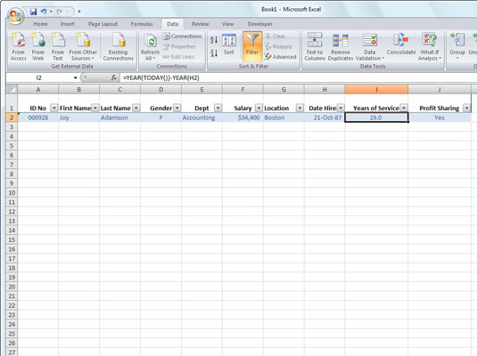
You can create a table in Excel 2007 (a list or database in previous Excel versions) to help you manage and analyze related data. The purpose of an Excel table is not so much to calculate new values but rather to store lots of information in a consistent manner, making it easier to format, sort, and filter worksheet data. Typically, an Excel table has only column headings and no row headings.

An Excel table is not the same as a data table that can be used for what-if analysis. You use a data table to show how changing one or two variables in formulas affects the results of those formulas.

1

Enter your table's column headings.

Click the blank cell where you want to start the new table and then enter the column headings (such as ID No, First Name, Last Name, Dept, and so on) in separate cells within the same row. Column headings are also known asfield names. The column headings should appear in a single row without any blank cells between the entries.

2

Enter the first row of data immediately below the column headings you typed in Step 1.

These entries constitute the first row, or record, of the table.

3

Click the Table command button in the Tables group of the Insert tab.

Excel displays a marquee around all the cells in the new table. The Create Table dialog box appears, listing the address of the table in the Where Is the Data for Your Table text box. (If the address displayed here is incorrect, drag in the worksheet to select the correct range.)

4

Click the My Table Has Headers check box to select it.

These headers are the column headings entered in the first step.

 Enlarge

5

Click OK.

Excel inserts and formats the new table and adds filter arrows (drop-down buttons) to each of the field names in the top row.

Another way to insert a table is to click the Format as Table button in the Styles group on the Home tab and then select a table style of your choice in the gallery that appears. Use this method if you want to apply a different table style as you create a table.

If you want to convert an existing Excel table back to a normal range of cells, select any cell in the table and then click the Convert to Range button on the Table Tools Design tab. All data and formatting is preserved

Question 2 - Give examples for Mathematics formula using Exce

Excel Formulas Overview

This tutorial covers in detail how to create and use formulas, including a step by step example of a basic Excel formula. It is intended for those with little or no experience in working withspreadsheet programs such as Excel.

Click on the links below to read specific information.

1. Writing the Formula - How to enter a formula
2. Cell References in Formulas - Make it easy to change your spreadsheet
3. Updating Excel Formulas - Automatic updating
4. Mathematical Operators in Formulas- Adding to formulas
5. Excel Formulas Tutorial Step 1- Entering the Data
6. Excel Formulas Tutorial Step 2 - Add the Equal (=) Sign
7. Excel Formulas Tutorial Step 3 - Add Cell References Using Pointing

Writing the Formula

Writing Excel formulas is a little different than the way it is done in math class.

Excel formulas starts with the equal sign ( = ) rather than ending with it.

The equal sign always goes in the cell where you want the formula answer to appear.

The equal sign informs Excel that what follows is part of a formula, and not just a name or a number.

Excel formulas look like this:

=3 + 2

rather than:

3 + 2 =

Cell References in Formulas

While the formula in the previous step works, it has one drawback. If you want to change the data being calculated you need to edit or rewrite the formula.

A better way would be to write formulas so that you can change the data without having to change the formulas themselves.

To do this, you need to tell Excel which cell the data is located in. A cell's location in the spreadsheet is referred to as its cell reference.

To find a cell reference, simply look at the column headings to find which column the cell is in, and across to find which row it is in.

The cell reference is a combination of the column letter and row number -- such as A1, B3, orZ345. When writing cell references the column letter always comes first.

So, instead of writing this formula in cell C1:

= 3 + 2

write this instead:

= A1+A2

Note: When you click on a cell containing a formula in Microsoft Excel (see the example above), the formula always appears in the formula bar located above the column letters (circled in red in the example).

 

Updating Excel Formulas

When you use cell references in Excel formulas, the formulas will automatically update whenever the relevent data in the spreadsheet changes.

For example, if you realize that the data in cell A1 should have been an 8 instead of a 3, you only need to change the contents of cell A1.

Excel updates the answer in cell C1. The formula, itself, doesn't need to change because it was written using cell references.

Changing the data

1. Click on the cell A1
2. Type an 8
3. Press the ENTER key on the keyboard

The answer in cell C1 where the formula is, immediately changes from 5 to 10, but the formula itself is unchanged.

Mathematical Operators

Creating formulas in Microsoft Excel is not difficult. Just combine the cell references of your data with the correct mathematical operator.

The mathematical operators used in Excel formulas are similar to the ones used in math class.

• Subtraction - minus sign ( - )
• Addition - plus sign ( + )
• Division - forward slash ( / )
• Multiplication - asterisk (* )
• Exponentiation - caret (^ )

Order of Operations

If more than one operator is used in a formula, there is a specific order that Excel will follow to perform these mathematical operations. This order of operations can be changed by adding brackets to the equation. An easy way to remember the order of operations is to use the acronym:

BEDMAS

The Order of Operations is:

Brackets
Exponents
Division
Multiplication
Addition
Subtraction

How the Order of Operations Works

Any operation(s) contained in brackets will be carried out first followed by any exponents.

After that, Excel considers division or multiplication operations to be of equal importance, and carries out these operations in the order they occur left to right in the equation.

The same goes for the next two operations – addition and subtraction. They are considered equal in the order of operations. Which ever one appears first in an equation, either addition or subtraction, is the operation carried out first.

Excel Formulas Tutorial Step 1: Entering the Data

Let's try a step by step example. We will write a simple formula in Excel to add the numbers 3 + 2.

Step 1: Entering the data
It's best if you first enter all of your data into the spreadsheet before you begin creating formulas. This way you will know if there are any layout problems, and it is less likely that you will need to correct your formula later.

For help with this tutorial refer to the image above.

1. Type a 3 in cell A1 and press the ENTER key on the keyboard.
2. Type a 2 in cell A2 and press the ENTER key on the keyboard.

Excel Formulas Tutorial Step 2: Add the Equal (=) Sign

When creating formulas in Microsoft Excel, you ALWAYS start by typing the equal sign. You type it in the cell where you want the answer to appear.

For help with this example refer to the image above.

1. Click on cell C1(outlined in black in the image) with your mouse pointer.
2. Type the equal sign in cell C1.

Excel Formulas Tutorial Step 3: Add Cell References Using Pointing

After typing the equal sign in step 2, you have two choices for adding cell references to the spreadsheet formula.

1. You can type them in or,
2. You can use an Excel feature called Pointing

Pointing allows you to click with your mouse on the cell containing your data to add its cell reference to the formula.

After typing an equal sign in cell C1 in step 2:

1. Click on cell A1 with the mouse pointer to enter the cell reference into the formula
2. Type a plus (+) sign
3. Click on cell A2 with the mouse pointer to enter the cell reference into the formula
4. Press the ENTER key on the keyboard

The answer 5 should appear in cell C1.

If you have more than one row or column of data that you need to perform calculations on, it is often possible to copy the first formula to other cells.

The easiest way to do this is to copy formulas with the fill handle.

Question 3 - How To insert Symbol RM with 2 Decimal Places 

1. Select the cell or range of cells that contains the numbers that you want to display with a currency symbol.

How to select a cell or a range

2. On the Format menu, click Cells.
3. On the Number tab, click Currency or Accounting in the Category box.
4. In the Symbol box, click the currency symbol that you want.

 NOTE   If you want to display a monetary value without a currency symbol, you can click None.

5. In the Decimal places box, enter the number of decimal places that you want to display.
6. In the Negative numbers box, select the display style for negative numbers.

 NOTE   The Negative numbers box is not available for the Accounting number format.

Tips

• To quickly display a number with the default currency symbol, select the cell or range of cells and then clickCurrency Style  on the Formatting toolbar.
• To change the default currency symbol for Excel and other Microsoft Office programs, you can change the default country/region settings in Control Panel. Note that although the Currency Style button  image does not change, the currency symbol that you chose will be applied when you click the button. For more information, see Change the default country/region.
• To reset the number format, click General in the Category box. Cells that are formatted with the Generalformat have no specific number format.

Conclusion

After do some exercise and calculation , finally i know how to calculate using Microsoft Excel and finished it ..